This will be a quick and dirty walkthrough of how to get results from a raw leaf physiognomic dataset.
Background
This package contains functions that enable the quick analysis of a quantitative leaf physiognomic dataset.
We provide a function for Digital Leaf Physiognomy
(dilp()), which estimates paleoclimate via multiple linear
regressions calibrated with a modern dataset.
We also provide functions for Leaf Margin Analysis
(temp_slr()) and Leaf Area Analysis
(precip_slr()), simple linear regressions that estimate
mean annual temperature (MAT) and mean annual precipitation (MAP)
respectively.
Lastly, we provide a function for reconstructing fossil leaf mass per
area (lma()), a functional trait that reflects leaf
resource economy.
In this vignette, we’ll walk you through the standard workflow for a
complete leaf physiognomic dataset, using the included
McAbeeExample dataset.
For ease of use, a template spreadsheet for data collection can be found here: DiLP Data Collection Template.
If you encounter any problems, or would like to request a feature, please create an issue on the github page.
# If the dataset is in good shape, this is all you need to do

dilp_results <- dilp(McAbeeExample)
#> Warning in dilp_outliers(processed_specimen_data): Outliers found. Please
#> evaluate $outliers for possible wrong measurements
lma_results <- lma(McAbeeExample)

# This just grabs the key data points from the results
data.frame(
  Site = c("McAbee H1", "McAbee H2"),
  MAT_MLR = dilp_results$results$MAT.MLR,
  MAT_SLR = dilp_results$results$MAT.SLR,
  MAP_MLR = dilp_results$results$MAP.MLR,
  MAP_SLR = dilp_results$results$MAP.SLR,
  site_mean_LMA = lma_results$lowe_site_mean_lma$value
)
#>        Site  MAT_MLR  MAT_SLR  MAP_MLR  MAP_SLR site_mean_LMA
#> 1 McAbee H1 13.54419 11.18065 106.7353 126.7697      73.68178
#> 2 McAbee H2 11.63970  9.36000 133.6330 135.8734      67.58568
And that’s basically it! Climate estimates and associated information
can be found in the output generated by dilp(), and leaf
mass per area reconstructions can be found in the output generated by
lma().
Read on for a breakdown of key DiLP and LMA components and helper functions.
DiLP Paleoclimate Estimates in Depth
To go a bit more in depth, if the dataset is correctly formatted, all
that needs to be done is to pass it through the dilp()
function, which takes the following steps to produce paleoclimate
estimates.
First, the data is processed using the dilp_processing()
function, which cleans up the raw dataset and generates derived
physiognomic characters based on the raw physiognomic data.
Next, possible errors and outlier measurements are identified using
the dilp_errors() and dilp_outliers()
functions.
Finally, Mean Annual Temperature (MAT) and Mean Annual Precipitation (MAP) are estimated using both multiple and simple linear regressions. Default parameters used are from the global regressions provided by Peppe et al. (2011).
All this information will be contained within the returned list.
# Elements of DiLP results:
print(paste0("dilp_results$", names(dilp_results)))
#> [1] "dilp_results$processed_leaf_data"
#> [2] "dilp_results$processed_morphotype_data"
#> [3] "dilp_results$processed_site_data"
#> [4] "dilp_results$errors"
#> [5] "dilp_results$outliers"
#> [6] "dilp_results$results"
After generating dilp() results, make sure to check
whether any common errors were discovered within the dataset.
There are no errors in the McAbeeExample dataset, but if
there were, this table would identify the specimens in the original
dataset that triggered the errors.
dilp_results$errors
#>                                                   Check specimen_number
#> 1                             Entire tooth count not NA No errors found
#> 2                        Entire tooth count : IP not NA No errors found
#> 3                         Entire perimeter ratio not NA No errors found
#> 4                                   FDR not between 0-1 No errors found
#> 5 External perimeter not larger than internal perimeter No errors found
#> 6                Feret is not larger than minimum Feret No errors found
#> 7                           Perimeter ratio less than 1 No errors found
Similarly, check if there are any outlier datapoints. These aren’t necessarily errors, but it may be worth double checking the original measurements.
In the McAbeeExample dataset, three specimens are
identified as outliers in tooth count:internal perimeter ratio, three
specimens are outliers in leaf area, and four specimens are outliers in
perimeter ratio. In this case, each of these were re-examined and found
to be acceptable outliers.
dilp_results$outliers
#>         site specimen_number morphotype outlier.entire.dataset
#> 1  McAbee H1    BU-712-1073A        M28        perimeter_ratio
#> 2  McAbee H1     BU-712-1117         M8                  tc_ip
#> 3  McAbee H1     BU-712-1165        M28        perimeter_ratio
#> 4  McAbee H1    BU-712-1169A         M8                  tc_ip
#> 5  McAbee H1    BU-712-1176A         M8                  tc_ip
#> 6  McAbee H1    BU-712-1182A         M5            No outliers
#> 7  McAbee H1    BU-712-1182A         M5            No outliers
#> 8  McAbee H1      M-2015-1-1        M24        perimeter_ratio
#> 9  McAbee H1    M-2015-1-122         M5            No outliers
#> 10 McAbee H1     M-2015-1-17        M28            No outliers
#> 11 McAbee H1      M-2015-1-3         M5            No outliers
#> 12 McAbee H1      M-2015-1-3         M5            No outliers
#> 13 McAbee H1     M-2015-1-40         M5            No outliers
#> 14 McAbee H1     M-2015-1-62        M28        perimeter_ratio
#> 15 McAbee H1     M-2015-1-69         M8            No outliers
#> 16 McAbee H1      M-2015-1-7        M19            No outliers
#> 17 McAbee H2    BU-712-2105A        M47              leaf_area
#> 18 McAbee H2     BU-712-2124        M94              leaf_area
#> 19 McAbee H2    BU-712-2173A        M18              leaf_area
#> 20 McAbee H2     BU-712-2197        M19            No outliers
#> 21 McAbee H2     M-2015-2-15        M19            No outliers
#> 22 McAbee H2     M-2015-2-84        M19            No outliers
#>    outlier.morphotype
#> 1         No outliers
#> 2               tc_ip
#> 3         No outliers
#> 4               tc_ip
#> 5               tc_ip
#> 6               tc_ip
#> 7     perimeter_ratio
#> 8     perimeter_ratio
#> 9     perimeter_ratio
#> 10    perimeter_ratio
#> 11              tc_ip
#> 12    perimeter_ratio
#> 13    perimeter_ratio
#> 14    perimeter_ratio
#> 15    perimeter_ratio
#> 16              tc_ip
#> 17        No outliers
#> 18        No outliers
#> 19        No outliers
#> 20    perimeter_ratio
#> 21              tc_ip
#> 22              tc_ip
Now, let’s take a look at the results. Paleoclimate reconstructions will be generated for each unique site found within the dataset.
The Margin, FDR, TC.IP, Ln.leaf.area, Ln.TC.IP, and Ln.PR columns simply report the site-level values for the parameters used in the DiLP regressions. The MAT.MLR and MAP.MLR columns report the temperature and precipitation results using those parameters. The MAT.SLR and MAP.SLR columns report temperature and precipitation results using simple linear regressions. Positive and negative error for all paleoclimate estimates are reported as well.
dilp_results$results
#>        site   margin       fdr    tc_ip ln_leaf_area  ln_tc_ip     ln_pr
#> 1 McAbee H1 32.25806 0.6965086 2.562487     6.792833 0.6070757 0.2047427
#> 2 McAbee H2 23.33333 0.7012671 2.651242     7.037892 0.6218561 0.1504205
#>    MAT.MLR MAT.MLR.error  MAT.SLR MAT.SLR.error  MAP.MLR MAP.MLR.error.plus
#> 1 13.54419             4 11.18065           4.8 106.7353           87.74914
#> 2 11.63970             4  9.36000           4.8 133.6330          109.86219
#>   MAP.MLR.error.minus  MAP.SLR MAP.SLR.error.plus MAP.SLR.error.minus
#> 1            48.15775 126.7697           106.5412            57.88926
#> 2            60.29365 135.8734           114.1923            62.04646
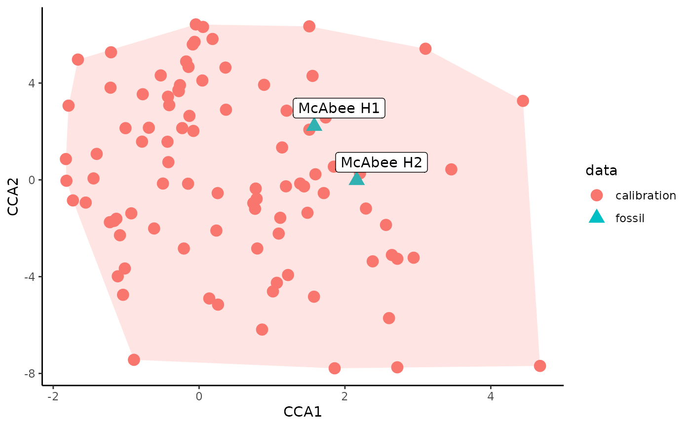
Next, dilp_cca() can be called to make sure that your
sites fit within the physiognomic space encompassed by the calibration
data.
dilp_cca(dilp_results)
If a site you are testing falls outside the bounds of the calibration data, the DiLP regressions may not be able to accurately reconstruct the paleoclimate of that site.
In this case, both McAbee localities do fall within the bounds of the calibration data; thus, the use of DiLP is appropriate here.
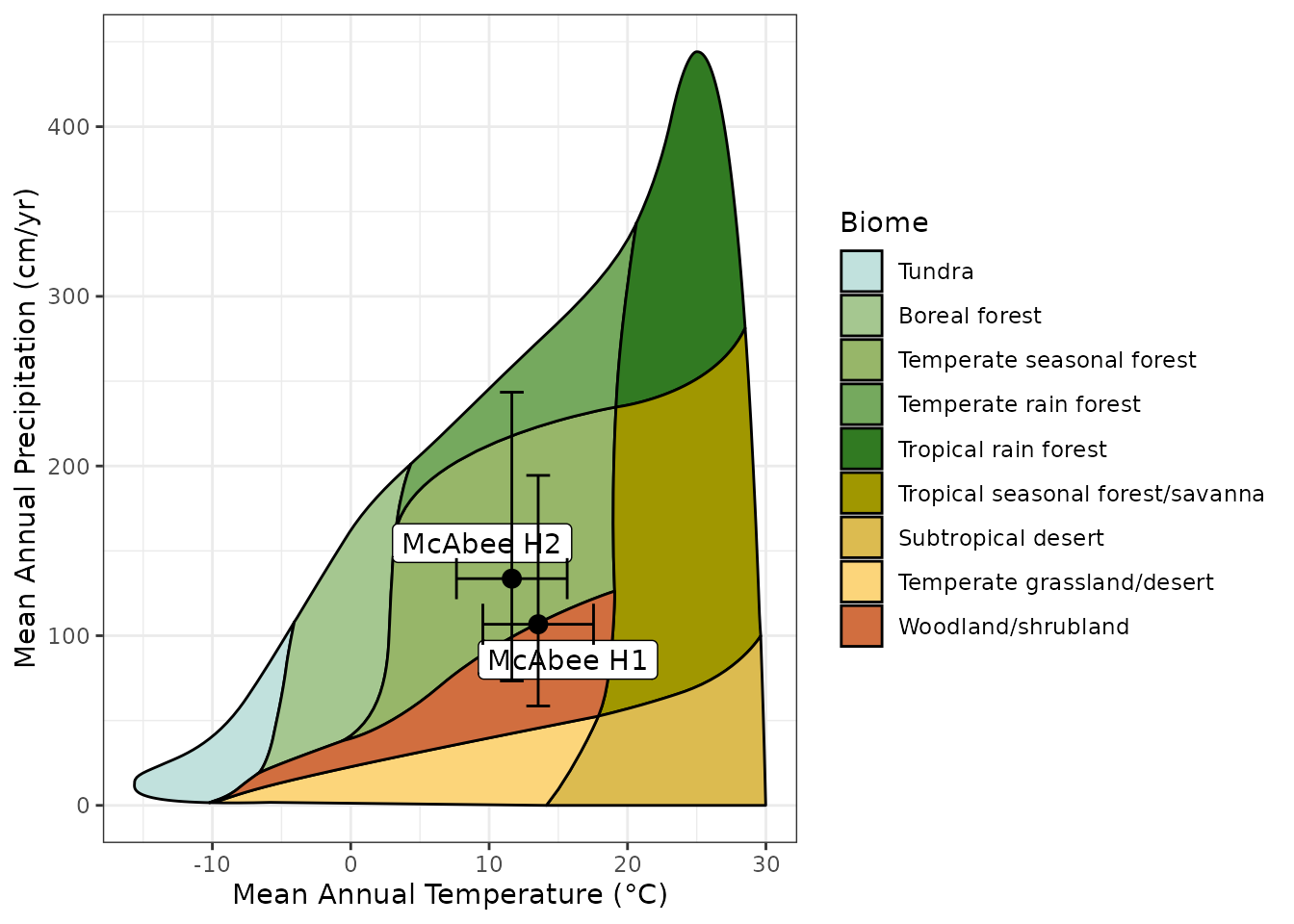
Finally, dilp_whittaker() can be called to visualize the
Whittaker Biome placement of each site as well as the errorbars for
paleoclimate reconstructions.
dilp_whittaker(dilp_results)
Leaf Mass per Area Reconstructions in Depth
Leaf mass per area reconstructions can be generated from a smaller subset of leaf physiognomic data than is needed for DiLP paleoclimate estimates. All you really need is leaf area and petiole width.
The standard suite of DiLP traits already includes leaf area and
petiole width, so here we will just continue using the included
McAbeeExample dataset.
lma_results <- lma(McAbeeExample)
print(paste0("lma_results$", names(lma_results)))
#> [1] "lma_results$species_mean_lma"       "lma_results$royer_site_mean_lma"
#> [3] "lma_results$lowe_site_mean_lma"     "lma_results$lowe_site_variance_lma"
As with dilp(), results for lma() are saved
within a list. lma_results$species_mean_lma includes the reconstructed
mean LMA for every species-site pair in the dataset. Upper and lower
prediction intervals are calculated as well.
lma_results$species_mean_lma
#>         site morphotype  n petiole_metric    lower     value     upper
#> 1  McAbee H1         M1 10   0.0018166221 81.37167 105.44818 136.64852
#> 2  McAbee H1         M5  3   0.0011067149 54.54670  87.26130 139.59661
#> 3  McAbee H1         M8  8   0.0011510539 66.35987  88.58058 118.24193
#> 4  McAbee H1        M12  1   0.0010808383 38.37080  86.47620 194.89128
#> 5  McAbee H1        M13  1   0.0006070381 30.77894  69.37268 156.35916
#> 6  McAbee H1        M18  1   0.0011637972 39.46986  88.95393 200.47708
#> 7  McAbee H1        M19  1   0.0008073257 34.32356  77.35576 174.33838
#> 8  McAbee H1        M24  5   0.0002309535 33.24559  47.95859  69.18289
#> 9  McAbee H1        M28  1   0.0002175761 20.78085  46.87783 105.74787
#> 10 McAbee H1        M41  1   0.0002994371 23.48554  52.96009 119.42543
#> 11 McAbee H1        M44  1   0.0005108600 28.81385  64.94883 146.40011
#> 12 McAbee H1        M73  1   0.0003778943 25.67425  57.88359 130.50081
#> 13 McAbee H1        M79  2   0.0003960090 33.14315  58.92822 104.77386
#> 14 McAbee H1        M91  1   0.0001524066 18.12949  40.91735  92.34838
#> 15 McAbee H2         M1  3   0.0008877491 50.14134  80.21339 128.32102
#> 16 McAbee H2         M8  2   0.0010796906 48.64042  86.44111 153.61845
#> 17 McAbee H2        M18  1   0.0002132426 20.62123  46.51895 104.94097
#> 18 McAbee H2        M19  4   0.0006803596 48.21879  72.46130 108.89200
#> 19 McAbee H2        M22  3   0.0008971039 50.34260  80.53524 128.83571
#> 20 McAbee H2        M24  2   0.0007082087 41.40139  73.58031 130.77005
#> 21 McAbee H2        M28  1   0.0004553366 27.57296  62.15600 140.11437
#> 22 McAbee H2        M29  1   0.0001254609 16.82558  37.98658  85.76111
#> 23 McAbee H2        M31  2   0.0003283234 30.84620  54.85640  97.55577
#> 24 McAbee H2        M47  2   0.0009868057 46.99765  83.52115 148.42836
#> 25 McAbee H2        M76  1   0.0001534697 18.17789  41.02614  92.59292
#> 26 McAbee H2        M94  1   0.0001232820 16.71284  37.73320  85.19165
#> 27 McAbee H2        M97  1   0.0005314955 29.25363  65.93877 148.62843
Three different metrics of site level LMA are calculated.
royer_site_mean_lma and lowe_site_mean_lma use slightly different regressions to show the average LMA of all species at a site.
lowe_site_variance_lma shows the variance of species-mean LMA values at a site.
# Royer Site Mean LMA
lma_results$royer_site_mean_lma
#>        site  n    lower    value    upper
#> 1 McAbee H1 14 64.42873 72.90997 82.50765
#> 2 McAbee H2 13 57.33929 65.48619 74.79063
# Lowe Site Mean LMA
lma_results$lowe_site_mean_lma
#>        site  n    lower    value    upper
#> 1 McAbee H1 14 61.03750 73.68178 88.94539
#> 2 McAbee H2 13 53.87969 67.58568 84.77822
# Lowe Site Variance LMA
lma_results$lowe_site_variance_lma
#>        site  n    lower     value    upper
#> 1 McAbee H1 14 491.2574 1070.6851 2333.535
#> 2 McAbee H2 13 323.3496  866.6651 2322.899
Paleoclimate Estimates with Simple linear regressions
Sometimes, you may not have a full leaf physiognomic dataset recorded
for a site. In that case, simple linear regressions can be used to
estimate MAT (temp_slr()) and
MAP(precip_slr()) so long as you have margin state or leaf
area data, respectively.
See the documentation for either function to learn about the different regressions that are preloaded into the functions. In this case, we’ll use the Peppe2018 regression for MAT and the Wilf1998 regression for MAP.
temp_slr(McAbeeExample, regression = "Peppe2018")
#>        site  n    lower      MAT    upper
#> 1 McAbee H1 31 7.602065 12.14206 16.68206
#> 2 McAbee H2 30 5.870667 10.41067 14.95067
precip_slr(McAbeeExample, regression = "Wilf1998")
#>        site  n    lower       MAP    upper
#> 1 McAbee H1 17 27.07551  89.55803 217.9242
#> 2 McAbee H2 13 30.95183 102.37976 249.1237
You can also use your own regressions for both of these functions as long as you provide the slope, the constant, and the standard error .
temp_slr(McAbeeExample, slope = 0.290, constant = 1.320, error = 5)
#>        site  n    lower       MAT    upper
#> 1 McAbee H1 31 5.674839 10.674839 15.67484
#> 2 McAbee H2 30 3.086667  8.086667 13.08667